The concept of virtual instruments is simple and quick way see the result by simulating real events. The operating principle of all Multisim tools (connection to the circuit, use) is identical to the operating principle of real analogues of these devices. In order to add a virtual device to working field program, you need to use the left mouse button to click on its icon in the “Device” panel and place it using the mouse in the required place on the diagram. In order to display the front panel of the device, you need to double-click the left mouse button on the device icon in the diagram. Once the panel opens, make the necessary settings just as you would on a real instrument panel. The principle of connecting virtual instruments to circuit elements is the same as for other circuit components. Let's take a closer look at working with such virtual instruments as a logic analyzer and a Bode plotter.

Logic analyzer

A logic analyzer is a device designed to monitor the state of logical elements of digital electronic devices when developing large systems, as well as for troubleshooting. To pick up signals from the circuit under study, the logic analyzer has 16 pins. In addition, this virtual device is equipped with three trigger inputs: C (external synchronization), Q (selective trigger input), T (masked trigger input).

Let us demonstrate the operation of this device. To generate signals, we will use two functional generators, which we will configure in such a way that they generate rectangular pulses with different frequencies - in our case 1 kHz and 5 kHz. Let's connect the terminals of the functional generators to the signal terminals of the logic analyzer using conductors of different colors, as a result of which the rectangular pulses on the clock diagram of the logic analyzer will also be displayed different colors. Let's start the circuit simulation and open the front panel of the logic analyzer. The logic analyzer icon, connection to the circuit and its front panel are shown in Figure 1. Figure 2 shows the settings windows for the XFG1 and XFG2 function generators.

Rice. 1. Logic analyzer icon, connection to the circuit and its front panel

Rice. 2. Settings windows for function generators XFG1 and XFG2

Let's look at the front panel of the logic analyzer in more detail. Sixteen switches on the left side of the panel correspond to sixteen signal acquisition channels. The switches become active if the analyzer outputs are connected to the nodes digital circuit, otherwise, when the analyzer channels are free, the switches are inactive. The next column displays the names of the circuit nodes corresponding to the analyzer channels connected to them. After running the circuit simulation, the logic analyzer takes the input values ​​from its pins and displays the resulting data as square waves on a clock diagram in the time domain of the front panel. The output of values ​​begins with channel 1. The lower part of the time domain displays the signals received from the analyzer's trigger inputs. The device is also equipped with two cursors designed for taking measurements in the time domain. At the bottom of the front panel of the device in question there is a control panel, on the left side of which there are three buttons:

• “Stop” (stop analysis);
• “Reset” (clear the temporary area screen);
• “Screen” (invert the time domain screen color).

In the central part of the control panel there is a cursor display window, which contains three fields:

• “T1” (T1 cursor readings);
• “T2” (T2 cursor readings);
• “T2-T1” (time shift between cursors).

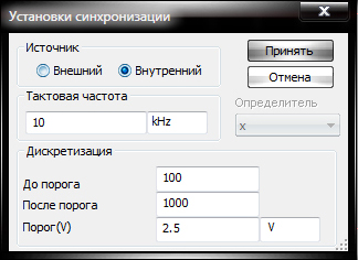
The arrow buttons allow you to change the cursor values ​​up or down. The cursor position code is displayed in the “Input Code” field, which is located behind the cursor readings field.

On the right side of the control panel there is a startup parameters window, in which in the “Time/Div” field you can set the number of clock cycles per division. Setting the input signal timing parameters can be done using the “Setup” button, which is located in the “Sweep” group of the launch parameters window. After clicking this button, the “Synchronization Settings” window will open (Fig. 3), in which the following parameters are configured:

• “Source” - source of clock pulses (external or internal), the parameter is set by setting the switch to the desired position;
• “Clock frequency” – set by entering a value from the keyboard into this field;
• “Determinant” – sets the active level of the synchronization signal (0 or 1);
• “Sampling” – parameters for sampling signals before the threshold, after the threshold, as well as the threshold value are set.

Rice. 3. “Synchronization Settings” window

Additional conditions for launching the analyzer are configured in the “Launch Settings” window (Fig. 4). This window can be called up from the launch parameters window using the “Setup” button, which is located in the “Level” group. In the window, a mask is configured, which is used to filter logical levels and synchronize input signals. For the changes to take effect, you must click on the “Accept” button.

Rice. 4. Launch Settings Window

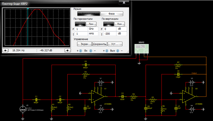
Bode plotter.

The Bode plotter is designed to analyze amplitude-frequency and phase-frequency characteristics and present them on a linear or logarithmic scale. This tool is most useful for analyzing filter circuits. A Bode plotter has four pins: two IN pins and two OUT pins. The device is connected to the circuit under study using the pins marked with the “+” sign (the IN pin “+” is connected to the input of the circuit, the OUT pin “+” is connected to the output), the pins “–” are connected to the common bus.

Let's take a closer look at the front panel of the device. On its left side there is a graphic display, which is designed to graphically display the signal shape. The device is also equipped with a cursor for taking measurements at any point on the graph; if necessary, the cursor can be moved using the left mouse button. You can also control the position of the cursor using the vertical cursor arrows, which are located in the lower left part of the front panel of the Bode plotter under the graphic display. Between the arrows there are two information fields that display the frequency and phase (or transmission coefficient) values ​​​​obtained at the intersection of the vertical cursor and the graph. On the right side there is a control panel designed to configure the parameters of the Bode plotter. Let's look at this panel in more detail. At the top of the panel there is a “Mode” field, which contains two buttons: “Amplitude” and “Phase”. When the “Amplitude” button is pressed, the device operates in the mode of analyzing amplitude-frequency characteristics. When the “Phase” button is pressed – in the phase-frequency characteristics analysis mode. In the “Horizontal” and “Vertical” fields, you can set the parameters of the horizontal and vertical coordinate axes on a logarithmic or linear scale. The logarithmic scale is used if the values ​​being compared have a large scatter, as, for example, in the case of analyzing the amplitude-frequency characteristics. The scale is switched using the “Log” (logarithmic) and “Lin” (linear) buttons. The scale of the horizontal (X-axis) and vertical (Y-axis) axes is determined by the initial (“I” - initial) and final (“F” - final) values. On the graphical display screen of a Bode plotter, the X axis always displays frequency. When measuring gain, the Y-axis displays the ratio of a circuit's output voltage to its input voltage. For a logarithmic scale, the units are decibels. If phase is measured, the vertical axis always shows the phase angle in degrees. When analyzing the amplitude-frequency response, the range of values ​​along the vertical axis can be set on a linear scale from 0 to 10e+09, on a logarithmic scale - from –200 dB to 200 dB. When analyzing the phase-frequency response, the range of values ​​along the vertical axis can be set from –720 degrees to +720 degrees. An example of connecting a Bode plotter to a filter circuit and the front panel of this device are shown in Figure 5.

Rice. 5. An example of connecting a Bode plotter to a filter circuit and the front panel of this device

There are three buttons in the “Control” field on the front panel of the device:

• “Screen” – this button is designed to invert the color of the graphic display (black/white);
• “Save” – the button is intended for saving measurement results to a file on disk in the .bod format (Bode plotter format) or .tdm (binary file);
• “Set...” - the button is designed to select the resolution of the Bode plotter. After clicking on the “Set…” button, the “Settings” dialog box opens (Fig. 6), in which in the “Resolution” field you can set the required number of resolution points in the range from 1 to 1000 and for the changes to take effect , click on the “Accept” button. At the bottom of the control panel of the Bode plotter there are four switches (“In +”, “In –”, “Out +”, “Out –”), which display the connection of the Bode plotter outputs to the circuit under study.

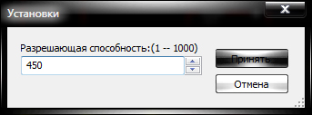
Rice. 6. “Settings” dialog box.

Before you run a circuit simulation in Multisim, you must ensure that the virtual instruments used in the circuit are configured correctly. This is an important note because in some cases, setting default parameters may not be appropriate for your design, and the user setting incorrect parameters may cause the results to be incorrect or difficult to read. If problems arise during circuit simulation, the errors that occur are recorded in an error and audit log file, which can be viewed by selecting Simulation/Analysis Log from the main Simulation menu. It should be noted that the settings of virtual instruments can also be changed during the simulation.

3.4 Frequency response and phase response meter (Bode Plotter)

The front panel of the frequency response-phase response meter is shown in Fig. 3.7. The meter is designed to analyze amplitude-frequency (with the MAGNI-TUDE button pressed, enabled by default) and phase-frequency (with the PHASE button pressed) characteristics with a logarithmic (LOG button enabled by default) or linear (LIN button) scale along the Y (VERTICAL) and X (HORIZONTAL). Setting up the meter consists of selecting the limits for measuring the transmission coefficient and frequency variation using the buttons in the F-maximum and I-minimum value boxes.

The device is connected to the circuit under study using the IN (input) and OUT (output) terminals. The left terminals of the clamps are connected, respectively, to the input and output of the device under test, and the right terminals are connected to the common bus. A function generator or other AC voltage source must be connected to the device input; no settings are required in these devices.

The EWB program uses a large set of instruments for carrying out measurements: ammeter, voltmeter, oscilloscope, multimeter, Bode Plotter ( Bode Plotter) (plotter of frequency characteristics of circuits), function generator, word generator, logic analyzer and logic converter.

The simplest devices in Electronics Workbench are a voltmeter and an ammeter, which are located in the indicator field ( Indicators) They do not require adjustment, automatically changing the measurement range. In one circuit, you can use several such devices simultaneously, observing currents in different branches and voltages on different elements.

Ammeter– used to measure variable and direct current rice. 2.6. The side of the rectangle representing the ammeter, highlighted with a thick line, corresponds to the negative terminal. By double-clicking on the ammeter image, a dialog box opens for changing the ammeter parameters: the type of current being measured, the value of internal resistance.

Rice. 2.6. Ammeter picture

The value of internal resistance is entered from the keyboard in the line Resistance , type of measured current (optional Mode ) is selected from the list. When measuring alternating sinusoidal current (AC), the ammeter will show its effective value

where is the amplitude value of the current.

The default internal resistance of 1 mOhm has a negligible effect on circuit operation in most cases. Its value can be changed, but using an ammeter with very low internal resistance in circuits with high output impedance may result in a mathematical error when simulating circuit operation. A multimeter can be used as an ammeter.

Voltmeter used to measure AC and DC voltage fig. 2.7.

Rice. 2.7. Voltmeter image

The side of the rectangle representing the voltmeter, highlighted with a thick line, corresponds to the negative terminal. Double-clicking on the voltmeter image opens a dialog box for changing the voltmeter parameters: the type of voltage being measured; the value of internal resistance. The value of internal resistance is entered from the keyboard in the line Resistance , type of measured voltage (optional Mode ) is selected from the list. When measuring alternating sinusoidal voltage (AC), the voltmeter will show the effective voltage value U, determined by the formula

Where – amplitude voltage value.

The voltmeter's default internal resistance of 1 MΩ has a negligible effect on circuit performance in most cases. Its value can be changed, but using a voltmeter with a very high internal resistance in circuits with low output impedance may result in a mathematical error when simulating circuit operation. You can use a multimeter as a voltmeter.

In addition to the ammeter and voltmeter described in Electronics Workbench There are seven devices, with numerous operating modes, each of which can be used only once in the circuit. These devices are located on the instrument panel. On the left side of the panel there are instruments for generating and observing analog quantities: a multimeter, a function generator, an oscilloscope, a Bode plotter (Fig. 2.8.:

Figure 2.8. Analog measuring instruments.

Multimeter used to measure: voltage (DC and AC), current (DC and AC), resistance, voltage level in decibels.

To configure the multimeter, you need to double-click on its reduced image to open its enlarged image (Fig. 2.9.

Rice. 2.9. Multimeter Images

a – reduced images for diagrams; b – enlarged image for setting up the multimeter.

In the enlarged image, by pressing the left mouse button, select: measured value by units of measurement – A, V, Ω or dB; type of measured signal - variable or constant; multimeter parameter setting mode. Setting the type of measured value is done by pressing the corresponding button on the enlarged image of the multimeter. Pressing a button with a symbol «~» sets the multimeter to measure the effective value alternating current and voltage, the DC component of the signal is not taken into account in the measurement. To measure direct voltage and current, you need to press the button with the symbol on the enlarged image of the multimeter « – ». As an ammeter and voltmeter, the multimeter is used in the same way as standard instruments.

Multimeter is the only standard instrument in Electronics Workbench designed for measuring resistance. To use a multimeter as an ohmmeter, connect it in parallel to the section of the circuit whose resistance you want to measure, press the button on the enlarged image of the multimeter Ω and a button with the “–” symbol to switch to the DC measurement mode. Enable schema. The measured resistance value will appear on the multimeter display.

To avoid erroneous readings, the circuit must have a connection to ground and no contact with power sources, which must be excluded from the circuit, the ideal current source being replaced by an open circuit and the ideal voltage source being replaced by a short circuit.

Oscilloscope, simulated by the program Workbench, is an analogue of a dual-beam storage oscilloscope and has two modifications:

1. a simple modification with the image of Fig. reduced to create a diagram. 2.10 A and an enlarged image for setting up the oscilloscope Fig. 2.10 b

Rice. 2.10. Simple modification oscilloscope

a – image of an oscilloscope in the circuit, b – oscilloscope panel for configuration

The advanced modification approaches in its capabilities the best digital storage oscilloscopes (Fig. 2.11.

Rice. 2.11. Advanced modification of the oscilloscope

Due to the fact that the extended model takes up a lot of space on the working surface, it is recommended to start research with a simple model, and to use an extended model for detailed research of processes.

The oscilloscope can be connected to an already turned on circuit or, while the circuit is running, you can rearrange the leads to other points - the image on the oscilloscope screen will change automatically. Double-clicking on the thumbnail image opens an image of the front panel of a simple oscilloscope model with control buttons, information fields and a screen.

To carry out measurements, the oscilloscope needs to be configured, for which you need to set:

· location of the axes along which the signal is deposited;

· the required scale of scanning along the axes;

· displacement of the origin of coordinates along the axes;

· input operating mode: closed or open;

· synchronization mode: internal or external.

The oscilloscope is configured using the control fields located on the control panel. The control panel is common to both modifications of the oscilloscope and is divided into four control fields:

horizontal scan ( Time base);

· synchronization ( Trigger);

· channel A;

· channel IN.

The horizontal scan (time scale) control field is used to set the scale of the horizontal axis of the oscilloscope when observing the voltage at the channel inputs A And IN depending on time. The time scale is specified in: s/div, ms/div, μs/div, ns/div (s/div, ms/div, ms/div, ns/div, respectively). The value of one division can be set from 0.1 ns to 1 s. The scale can be discretely decreased by one step when the mouse is clicked on the button to the right of the field and increased when the button is clicked.

Keystroke Expand in the simple model panel opens the oscilloscope advanced model window.

The panel of the extended model of the oscilloscope, in contrast to the simple model, is located under the screen and is supplemented by three information panels on which measurement results are displayed. In addition, directly below the screen there is a scroll bar, which allows you to observe any time period of the process from the moment of switching on to the moment of switching off the circuit. In essence, the extended model of an oscilloscope is a completely different device that allows you to carry out numerical analysis of processes much more conveniently and more accurately.

To return to the previous oscilloscope image, press the key Reduce located in the lower right corner.

Bode plotter(plotter) is used to obtain the amplitude-frequency (AFC) and phase-frequency (PFC) characteristics of the circuit in Fig. 2.12.

Rice. 2.12. Bode plotter images

a – reduced image for reflection in the diagram, b – enlarged for setting up the device

A Bode plotter measures the ratio of signal amplitudes at two points in a circuit and the phase shift between them. The amplitude ratio of signals can be measured in decibels. For measurements, the Bode plotter generates its own frequency spectrum, the range of which can be set when setting up the device. The frequency of any AC source in the circuit being tested is ignored, but the circuit must include some AC source.

The bode plotter has four terminals: two input ( IN) and two days off ( OUT). To measure the amplitude ratio or phase shift, you need to connect the positive terminals of the inputs IN And OUT(left terminals of the corresponding inputs) to the points under study, and ground the other two terminals. When you double-click on the reduced image of the Bode plotter (Fig. 2.12 A) its enlarged image opens (Fig. 2.12 b).

The top panel of the plotter specifies the type of characteristic obtained: frequency response or phase response. To obtain the frequency response, press the button Magnitude, to obtain the phase response – button Phase. Left control panel ( Vertical) sets:

· initial ( I– initial) and final ( F– final) values ​​of parameters plotted along the vertical axis,

· type of vertical axis scale – logarithmic ( LOG) or linear ( LIN).

Right control panel ( horizontal) is configured in the same way.

When obtaining the frequency response, the voltage ratio is plotted along the vertical axis:

· on a linear scale from 0 to 10 9 ;

· on a logarithmic scale from –200 dB to 200 dB.

When obtaining the phase response, degrees are plotted along the vertical axis: from –720 to +720. The horizontal axis always displays frequency in hertz or derived units.

The cursor is located at the beginning of the horizontal scale. It can be moved by clicking on the arrow buttons located to the right of the screen, or “dragged” using the mouse. The coordinates of the point of intersection of the cursor with the characteristic graph are displayed in the information fields at the bottom right. Using a Bode plotter, it is easy to construct a topographic diagram on the complex plane for any scheme.

Function generator is an ideal voltage source that produces sinusoidal, square or triangular signals (Fig. 2.13.

Rice. 2.13. Function generator image

a – reduced image to form a diagram. b – enlarged for tuning the generator.

The middle terminal of the generator, when connected to the circuit, provides a common point for measuring the amplitude of the alternating voltage. To measure the voltage relative to zero, the common terminal is grounded. The extreme right and left terminals are used to supply alternating voltage to the circuit. The voltage on the right terminal changes in a positive direction, and the voltage on the left terminal changes in a negative direction, relative to the common terminal.

When you double-click on the reduced image of the function generator, its enlarged image opens, with the help of which you can:

· setting the signal shape.

· setting the signal frequency.

· setting the output voltage amplitude.

· setting the constant component of the output voltage.

1 Setting the waveform. To select the required output signal shape, click on the button with the corresponding image. The shape of the triangle and square waveforms can be changed by decreasing or increasing the value in the field Duty Cycle(duty factor). This parameter is defined for triangle and square wave signals. For a triangular voltage waveform, it specifies the duration (as a percentage of the signal period) between the voltage rise interval and the fall interval.

By setting, for example, a value of 20, you can get the duration of the rising interval to be 20% of the period, and the duration of the falling interval to be 80%. For a rectangular voltage waveform, this parameter specifies the ratio between the durations of the positive and negative parts of the period.

2 Setting the signal frequency. The generator frequency is adjustable from 1 Hz to 999 MHz. The frequency value is set in the line Frequency using the keyboard and arrow keys. A numerical value is set in the left field, a unit of measurement is set in the right field (Hz, kHz, MHz - Hz, kHz, MHz, respectively).

3 Setting the output voltage amplitude. The output voltage amplitude can be adjusted from 0 mV to 999 kV. The amplitude value is set in the line Amplitude using the keyboard and arrow keys. The numerical value is set in the left field, the unit of measurement is set in the right field (mV, mV, V, kV - µV, mV, V, kV, respectively).

4 Setting the DC component of the output voltage. The DC component of the AC signal is set in line Offset using the keyboard or arrow keys. It can have both positive and negative meaning. This makes it possible to obtain, for example, a sequence of unipolar pulses.

Frequency response and phase response meter (Bode Plotter)

A Bode diagram meter (or Bode loss) is designed to measure the frequency response and phase response of electrical circuits.

The front panel of the frequency response-phase response meter (Bode diagram meter) is shown in Fig. 1.12.

The meter allows you to analyze the amplitude-frequency characteristics (with the MAGNITUDE button pressed, enabled by default) and phase-frequency (with the PHASE button pressed) characteristics with a logarithmic (LOG button enabled by default) or linear (LIN button) scale along the Y (VERTICAL) and X (HORIZONTAL). Setting up the meter consists of selecting the limits for measuring the transmission coefficient and frequency variation using the buttons in the windows A - maximum and I - minimum values. The frequency value and the corresponding transmission coefficient or phase value are displayed in the windows in the lower right corner of the meter.

The device is connected to the circuit under study using the IN (input) and OUT (output) terminals. The left terminals of the clamps are connected, respectively, to the input and output of the device under test, and the right terminals are connected to the common bus. A function generator or other AC voltage source must be connected to the device input; no settings are required in these devices.

2. Practical part

1. Measure the parameters of the harmonic oscillator signal using an oscilloscope and voltmeter. 1.1. Assemble the measurement circuit (Fig. 1.13).

1.1.1. Draw in the report a time diagram of a harmonic signal with amplitude U m = 5 V and frequency / = 2 kHz, showing the units of measurement along the axes, as well as the amplitude and period.

1.2. Set a harmonic signal with amplitude U M = 5 V and frequency /^ 2 kHz at the output of the i-generator.

1.3. Obtain on the oscilloscope screen a stable, unlimited from above, along the K axis, image of 2-3 periods of the harmonic signal within the entire screen along the X axis.

This is achieved by adjusting the sensitivity of channel A along the Y axis (B/Div switch), the sweep time on the X axis (Time/Div switch) and setting the oscilloscope to internal synchronization mode on channel A with the sweep starting at the positive edge of the input signal.

1.4. Measure the amplitude U m of the harmonic signal with an oscilloscope. Measuring the amplitude comes down to calculating it using the formula (Fig. 1.14)˸

Vm – K at, where N is the amplitude of the signal image in scale divisions along the Y axis, K is the scale factor along the K axis (the value of the V/Div switch).

It is much easier to measure the signal amplitude if you switch to the enlarged front panel mode of the oscilloscope (by pressing the ZOOM button). Measure the signal amplitude using the hairline and compare with the previously measured value.

1.5. Measure the amplitude of the harmonic signal with a voltmeter. The display of the multimeter shows the current (effective) value of the alternating voltage 1/l. Calculate the signal amplitude using the formula˸

and compare with what was measured earlier.

1.6. Measure the period using an oscilloscope and calculate the frequency of the signal under study. Measuring the period comes down to calculating ᴇᴦο using the formula (see Fig. 1.14)˸

Frequency response and phase response meter (Bode Plotter) - concept and types. Classification and features of the category "Frequency response and phase response meter (Bode Plotter)" 2015, 2017-2018.

The front panel of the frequency response-phase response meter is shown in Fig. 19. The meter is designed to analyze amplitude-frequency (with the MAGNITUDE button pressed, enabled by default) and phase-frequency (with the PHASE button pressed) characteristics with a logarithmic (LOG button, enabled by default) or linear (LIN button) scale along the Y axes (VERTICAL) and X (HORIZONTAL). Setting up the meter consists of selecting the limits for measuring transmission coefficient and frequency variation using the buttons in the windows F– maximum and I- minimum value.

The frequency value and the corresponding value of the transmission coefficient or phase are indicated in the windows in the lower right corner of the meter. The values ​​of the indicated quantities at individual points of the frequency response or phase response can be obtained using a vertical hairline, which is in the initial state at the origin of coordinates and is moved along the graph with the mouse or the ←, → buttons. The measurement results can also be written to a text file. To do this, click the SAVE button and specify the file name in the dialog box (by default, the name of the schematic file is suggested). In the text file “*.scp” obtained in this way, the frequency response and phase response are presented in tabular form.

Rice. 19. Frequency response and phase response meter.

The device is connected to the circuit under study using the IN (input) and OUT (output) terminals. The left terminals of the clamps are connected, respectively, to the input and output of the device under test, and the right terminals are connected to the common bus (ground). A function generator or other AC voltage source must be connected to the device input; no settings are required in these devices.

Spectrum analyzer

A spectrum analyzer is used to measure the amplitude of a harmonic with a given frequency. It can also measure signal power and frequency components, and determine the presence of harmonics in the signal. Spectrum analyzer results are displayed in the frequency domain rather than the time domain. Typically, the signal is a function of time, and an oscilloscope is used to measure it. Sometimes a sinusoidal signal is expected, but it may contain additional harmonics, making it impossible to measure the signal level. If the signal is measured by a spectral analyzer, the frequency composition of the signal is obtained, that is, the amplitude of the main and additional harmonics is determined.

Wattmeter.

The device is designed to measure power and power factor.

Current probe.

The current probe is designed to measure current values ​​in any part of the circuit of the simulated circuit.

Measuring probe.

Shows direct and alternating voltages and currents in a section of the circuit, as well as the frequency of the signal.